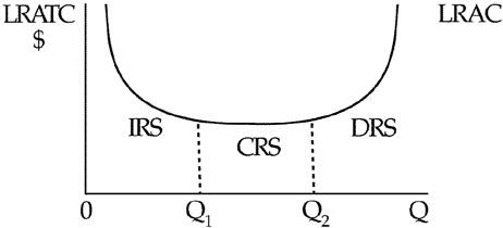
Draw a long-run average cost curve that first exhibits increasing returns to scale (economies of scale), then constant returns to scale, and finally decreasing returns to scale (diseconomies of scale). Label each region
Initially, LRAC declines as output increases when there are EOS (IRS). LRAC becomes flat when there are CRS. Finally, LRAC rises once DOS (DRS) set in. See Figure 7-20.
Figure 7-20
You might also like to view...
The purchase of government bonds by the Fed leads to a(n)
A) increase in the demand of bonds and a decrease in the price of bonds. B) increase in the supply of bonds and a decrease in bond prices. C) decrease in the demand of bonds and an increase in the price of bonds. D) decrease in the supply of bonds and an increase in bond prices.
Suppose that firms find that their inventories are less than planned. In this case, what is the initial relationship between aggregate planned expenditure and real GDP? Using the aggregate expenditure model, what adjustments, if any, take place?
What will be an ideal response?
If, at a firm's projected sales level, the marginal cost is $125, the average cost is $150 and the markup is 20 percent, then its selling price is
A) $125. B) $150. C) $165. D) $180.
Describe each of the following as a positive demand shock, a negative demand shock, a positive supply shock, or a negative supply shock, and specify how each are represented on the Phillips curve
a. a sudden increase in oil prices b. a large increase in spending on residential construction c. a sudden decrease in household wealth resulting from a stock market crash d. a substantial increase in productivity following technological advancements