Using a rectangular window of width 50 and a sampling rate of 10,000 samples/second, design an FIR digital filter to approximate the analog filter whose transfer function is
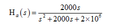
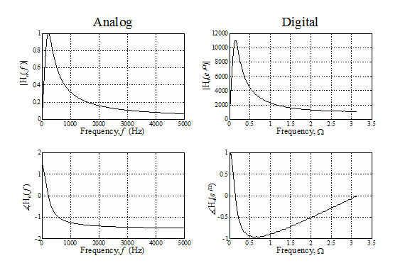
Compare the frequency responses of the analog and digital filters.
Inverse Laplace transforming we get the analog impulse response
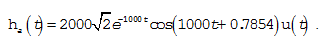
Sampling at 10,000 samples/second and truncating to 50 samples we get the impulse response of the digital FIR filter as

The easiest way to find the frequency response of the digital filter is to use the FFT in MATLAB.
%   Program to graph the frequency response of a windowed FIR filter with


%   50 samples sampled at 10 kHz to approximate an analog filter with


%   transfer function


%


%   Ha(s) = 2000s/(s^2+2000s+2e6)


%


close all ; figure('Position',[20,20,1500,800],'PaperPosition',[0.5,0.5,16,9.5]) ;


f = [0:20:5000]' ; %   Vector of cyclic frequencies


w = 2*pi*f ;       %   Vector of radian frequencies


s = j*w ;          %   Vector of s's


Ha = 2000*s./(s.^2+2000*s+2e6) ;    %   Analog filter freq resp


fs = 10000 ;                        %   Sampling rate


n = [0:49]' ;   %   Discrete-time vector for graphing


N = 50 ;        %   Length of impulse response


%   Generate the digital filter's impulse response


hd = 2000*sqrt(2)*(0.9048.^n).*cos(0.1*n+0.7854).*(uD(n) - uD(n-50)) ;


%   Extend the impulse response by a factor of padFac by zero padding


padFac = 8 ;    %   Zero padding factor


n = [0:padFac*N-1]' ;   %   Extend the impulse response time


hd = [hd;zeros((padFac-1)*N,1)] ;   %   Extend the impulse response


Hd = fft(hd) ;  %   Find the DTFT using the DFT


F = n/(padFac*N) ;  %   Vector of cyclic discrete-time frequencies


W = 2*pi*F ;        %   Vector of radian discrete-time frequencies


%   Graph the results


subplot(2,2,1) ;


ptr = plot(f,abs(Ha),'k') ; set(ptr,'LineWidth',2) ; grid on ;


xlabel('Frequency, {\itf}  (Hz)','FontName','Times','FontSize',24) ;


ylabel('|H_{\ita}( {\itj}2\pi{\itf} )|','FontName','Times','FontSize',24) ;


title('Analog','FontName','Times','FontSize',36) ;


set(gca,'FontName','Times','FontSize',18) ;


subplot(2,2,3) ;


ptr = plot(f,angle(Ha),'k') ; set(ptr,'LineWidth',2) ; grid on ;


xlabel('Frequency, {\itf}  (Hz)','FontName','Times','FontSize',24) ;


ylabel('Phase of H_{\ita} ( {\itj}2\pi{\itf} )','FontName','Times','FontSize',24) ;


set(gca,'FontName','Times','FontSize',18) ;


W = W(1:padFac*N/2) ; Hd = Hd(1:padFac*N/2) ;


subplot(2,2,2) ;


ptr = plot(W,abs(Hd),'k') ; set(ptr,'LineWidth',2) ; grid on ;


xlabel('Frequency, {\Omega}','FontName','Times','FontSize',24) ;


ylabel('|H_{\itd} ({\ite}^{{\itj}\Omega})|','FontName','Times','FontSize',24) ;


title('Digital','FontName','Times','FontSize',36) ;


set(gca,'FontName','Times','FontSize',18) ;


subplot(2,2,4) ;


ptr = plot(W,angle(Hd),'k') ; set(ptr,'LineWidth',2) ; grid on ;


xlabel('Frequency, {\Omega}','FontName','Times','FontSize',24) ;


ylabel('Phase of H_{\itd} ({\ite}^{{\itj}\Omega})','FontName','Times','FontSize',24) ;


set(gca,'FontName','Times','FontSize',18) ;


print -depsc -adobecset 'temp' ;
You might also like to view...
What kind of line is the line identified as B shown in Figure 1?
a. Hidden line b. Center line c. Visible line d. Section line
A board foot is a piece of planed wood 1-foot long, 1-foot wide, and 1-inch thick
Indicate whether the statement is true or false
The term used to designate the size of a nail is ____________________ and the symbol is ____________________.
Fill in the blank(s) with the appropriate word(s).
Imagine the company that you work for borrows $8,000,000 at 8% interest, and the loan is to be paid in seven years according to the schedule shown. Determine the amount of the last payment.
Year Amount 1 $1,000,000 2 $1,000,000 3 $1,000,000 4 $1,000,000 5 $1,000,000 6 $1,000,000 7 $?