Solve the set of difference equations derived in Problem 4.52 given the following values of the problem parameters
k = 40.0 W/(mK), disk thermal conductivity
a = 1 ? 10–5 m2/s, disk thermal diffusivity
Rs = 25 mm, disk radius
Zs = 5 mm, disk thickness
q" max = 3 x 10⁶ W/m2, peak absorbed flux
Ro = 50 mm, parameter in flux distribution
Tinit = 20°C, disk initial temperature
Determine the temperature distribution in the disk when the maximum temperature is 300°C.
GIVEN
- Difference equations developed in Problem 4.52 given the following values of the problem
parameters
FIND
(a) Disk temperature distribution when the maximum temperature is 300°C
All 9 difference equations can be written in the form
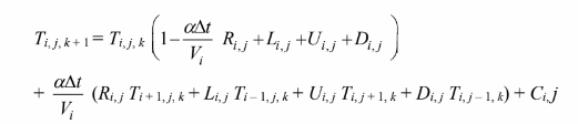
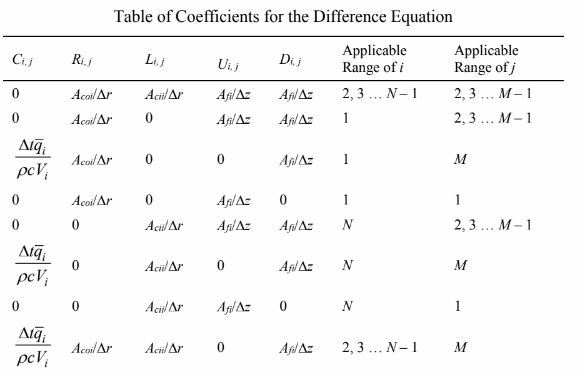
Where the coefficients Ci, j, Ri, j, Li, j, Ui, j, Di, j are defined in the table below. Note that to use the above
general equation for all nodes, we must allow the matrix of node temperatures to extend to indices
i = 0, i = N + 1, j = 0, and j = M + 1. Temperatures at these nodes do not have meaning, but to apply
the general difference equation along the axis or on the boundaries, they must be defined. Their values
do not matter because the coefficients are set up to account for the special equations on the axis or on
the boundaries.

To maintain a positive coefficient on Ti, j, k for stability we must have
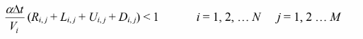
The largest permissible time step ?t is therefore
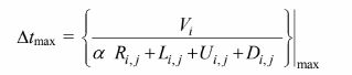
We will use some fraction of this time step in the program execution.
Note that we must first calculate the coefficients R, L, U, and D before determining ?tmax. Then we can
fill in the coefficients C.
The Pascal program listed below solves the difference equations as described above.
Program Prob3_M; {solution to Problem 3_M}


uses crt, printer;


const N = 11; {radial nodes}


M = 21; {axial nodes}


k = 40.0; {thermal conductivity (W/mK)}


alpha = 1e–5; {thermal diffusivity (m^2/s)}


Rs = 0.025; {disk radius (m)}


Zs = 0.005; {disk thickness (m)}


qmax = 3.0e6; {peak flux (W/m^2)}


Ro = 0.05; {parameter in flux equation (m)}


Tinit = 20.0; {initial temperature (C)}


Tmax = 300.0; {maximum desired temperature at top of axis (C)}


var dr, dz, rhoC, dtMax, dt, time:real;


i, j : integer;


C,R,L,U,D : array [1..N,1..M] of real;


q,V,Aco,Aci,Af : array [1..N] of real;


Toid,Tnew : array [1..N+1,1..M+1] of real;


begin


{calculate size of the control volumes}


dr : = Rs/(N – 1);


dz : = Zs/(M – 1);


rhoC: = k/alpha;


{calculate control volume surface areas and volumes}


Af[1] : = pi*dr*dr/4.0;


Af[N] : = pi*dr*(Rs – dr/4.0);


for i : = 2 to N – 1 do Af[i] : = 2.0*pi*dr*dr*(i – 1);


for i : = 1 to N do V[i] : = Af[i]*dz;


Aco[N] : = 2.0*pi*Rs*dz;


for i : = 1 to N – 1 do Aco[i] : = 2.0*pi*dr*dz*(i – 0.5);


Aci[1] : = 0.0;


for i : = 2 to N do Aci[i] : = 2.0*pi*dr*dz*(i – 1.5);


{calculate absorbed flux as function of i}


q [1] : = pi/4.0*qmax*dr*dr*(1.0 – 0.9/8.0*sqr(dr/Ro));


q [N] : = pi*qmax*dr*dr*(N – 1.25–0.9/8.0*sqr(dr/Ro)*(2.0*N*N*N –7.5*N*N


+ 9.5*N – 65.0/16.0));


for i : = 2 to N – 1 do


q [i] : = pi*qmax*dr*dr*(2.0*(1 – 1.0) – 0.9/4.0*sqr(dr/Ro)*(4.0*i*i*i – 12.0*i*


i + 13.0*i – 5.0));


{fill in the coefficient matrices}


for i : = 1 to N do {first, zero all of them out}


for j : = 1 to M do


begin


R[i, j] : = 0.0;


L[i, j] : = 0.0;


U[i, j] : = 0.0;


D[i, j] : = 0.0;


C[i, j] : = 0.0;


end


for i : = 2 to N – 1 do


for j : = 2 to M – 1 do


begin


R[i, j] : = Aco[i]/dr;


L[i, j] : = Aci[i]/dr;


U[i, j] : = Af[i]/dz;


D[i, j] : = Af[i]/dz;


end;


i : = 1;


for j : = 2 to M – 1 do


begin


R[i, j] : = Aco[i]/dr;


U[i, j] : = Af[i]/dz;


D[i, j] : = Af[i]/dz;


end;


i : = 1;


j : = M;


R[i, j] : = Aco[i]/dr;


D[i, j] : = Af[i]/dz;


i : = 1;


j : = 1;


R[i, j] : = Aco[i]/dr;


U[i, j] : = Af[i]/dz;


i : = N;


for j : = 2 to M – 1 do


begin


L[i, j] : = Aci[i]/dr;


U[i, j] : = Af[i]/dz;


D[i, j] : = Af[i]/dz;


end;


i : = N;


j : = M;


L[i, j] : = Aci[i]/dr;


D[i, j] : = Af[i]/dz;


i : = N;


j : = 1;


L[i, j] : = Aci[i]/dr;


U[i, j] : = Af[i]/dz;


j : = M;


for I : = 2 to N – 1 do


begin


R[i, j] : = Aco[i]/dr;


L[i, j] : = Aci[i]/dr;


D [i, j] : = Af[i]/dz;


end;


j : = 1;


for I : = 2 to N – 1 do


begin


R [i, j] : = Aco[i]/dr;


L [i, j] : = Aci[i]/dr;


U [i, j] : = Af[i]/dz;


end;


{find maximum permissible dt}


dtMax : = 0.0;


for i : = 1 to N do


for j : = 1 to M do


begin


dt : = V[i]/alpha/(R[i, j] + L[i, j] + U[i, j] + D[i, j]);


if = dt > dtMax then dtMax : = dt;


end;


dt : = 0.5*dtMax; {actual value to be used in solution}


{fill in the cij matrix}


for i : = 1 to N do C[i, M] : = dt*q [i]/rhoC/V[i];


{establish the initial conditions}


for i : = 1 to N do


for j : = 1 to M do


Told [i, j] : = Tinit;


{carry out the solution}


time : = 0.0;


repeat


time: = time + dt;


writeln (time: 10:5);


for i: = 1 to N do


for j: = 1 to M do


Tnew [i,j] : = Told [i,j]*(1.0 – alpha*dt/V[i]*(R[i,j]+ L[i,j]+ U[i,j]+


D[i,j))


+ alpha*dt/V[i]*(R[i, j]*Told [i + 1, j] + L[i, j]*Told [i – 1, j] + U[i, j]*Told


[i, j + 1] + D[i, j]*Told [i, j – 1]) + C[i, j];


if Tnew[1, m] > Tmax then {print out distribution and quit}


begin


writeln(1st, time : 8 : 4, ‘sec dt = ‘, dt : 15 : 10);


write(1st,’ ’);


for i : = 1 to N do write (1st, 1 : 10);


writeln(1st);


for j : = M downto 1 do


begin


write(1st, j : 4);


for i : = 1 to N do write(1st, Tnew[i, j]; 10 : 5);


writeln(1st);


end;


writeln(1st);


halt;


end


(otherwise, keep going}


for i : = 1 to N do


for j : = 1 to M do


Told[i, j] ; = Tnew[i, j];


until time < - 1.0;


end.
Now, we need to determine the node spacing and ?t required for an accurate solution. As suggested in
the text, trial and error is the best method.
First, let’s determine the required spatial resolution, that is, the values of N and M. Since the gradients
in the radial direction are small compared to those in the axial direction, we don’t expect much
influence on the results by varying N so we will use N = 11. Now, pick values of M = 11, 21, 41, and
61. A time step of ?t = 0.0003 s will give stable results for all these values of M. The table below gives
the results for these 4 runs.
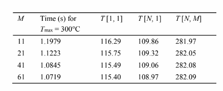
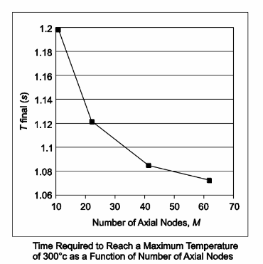
Notice that the temperatures in the table are not significantly affected by M but the time required to
reach 300°C is somewhat sensitive. This is displayed in the graph shown to the right. It appears that
the time gradually decreases but between M = 41 and M = 61, the graph levels off significantly. At
M = 81, the time would probably be somewhat less than that at M = 61 but clearly we have reached the
point of diminishing return. We will choose M = 41 as begin a reasonable compromise.
Next, we need to determine the appropriate time step, ?t. For N = 11, M = 41, the maximum
permissible time step according to the equation given previously is 0.00155 s. In practice, values larger
than 1/2 of this maximum result in instability. Running with 0.00015, 0.0003, and 0.0006 seconds, we
find
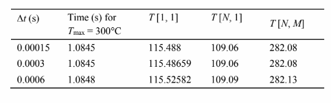
From the results in the table, it is clear that there is little benefit from a time step of less than 0.0003 s.
For a reasonable compromise, choose ?t = 0.0006 s.
Using these choices, M = 41, N = 11, and ?t = 0.0006 s, the results are plotted below
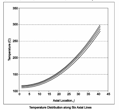
The solution shows that 1.0848 seconds is required for the maximum temperature in the disk to reach
300°C. Furthermore, the graph demonstrates that the temperature gradient axially through the disk is
not especially large as was required for the case hardening application. This indicates that the incident
flux needs to be increased.
You might also like to view...
When you are scuba diving, the pressure on your face plate
A) is independent of both depth and orientation. B) will be greatest when you are facing downward. C) depends only on your depth, and not on how you are oriented. D) will be greatest when you are facing upward.
In a particular case of Compton scattering, a photon collides with a free electron and scatters backwards. The wavelength after the collision is exactly double the wavelength before the collision. What is the wavelength of the incident photon?
A) 3.6 × 10⁻¹² m B) 4.8 × 10⁻¹² m C) 2.4 × 10⁻¹² m D) 1.2 × 10⁻¹² m E) 6.0 × 10⁻¹² m
A magnifying glass with focal length 15 cm is placed 10 cm above a stamp. The image of the stamp is located 30 cm above the magnifying glass
a. True b. False Indicate whether the statement is true or false
Due to the dual nature of light and matter, either can act in an experiment as if it is a wave or a particle. In which experiment is the wave aspect exhibited for matter?
a. the Davisson and Germer experiment b. the photoelectric effect c. pair production d. Compton scattering