Suppose all firms in an industry have a production technology described by the production function 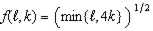 . The cost of labor is 2 and the cost of capital is 4, and each firm faces a recurring fixed cost of 300.
a. Derive the long run cost and average cost functions for each firm. (Hint: Given the shapes of the isoquants implied by the production function, you should be able to do this without solving a calculus problem.)
b. What is the long run equilibrium output price?
c. How much does each firm produce in long run equilibrium?
d. Suppose market demand is given by  . How many firms are in the industry in long run equilibrium?
e. Suppose the industry is currently in long run equilibrium. Derive the short run cost function for each firm (assuming labor is variable but capital is fixed in the short run).
f. Now suppose that demand falls to  . What happens to output price in the short run? What happens to price and the number of firms in the long run?
What will be an ideal response?
 units of labor and
  unit of capital. Thus, the cost of the inputs for x units of output is given by
 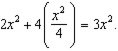 Including the recurring fixed cost, we then get a cost function of
 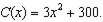 This implies an average cost function of
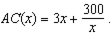
b. The long run output price occurs at the lowest point of the firms' AC curve -- i.e. where the derivative of AC(x) is zero. Solving
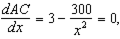 we get x=10, and plugging this back into the AC function, we get a long run equilibrium price of 60.
c. We just calculated in (b) that each firm produces 10 units of output in long run equilibrium.
d. At the long run equilibrium price of 60, the quantity demanded is 400. With each firm producing 10, this implies 40 firms in the industry.
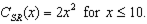
e. Since each firm is producing 10 in the LR equilibrium, each firm is using 100 units of labor and 25 units of capital. In the short run, firms can't produce more than 10 units of output (because of the extreme complementarity of inputs in production), but it can produce less by hiring less labor. The short run cost function for output is then
f. The short run market supply curve is the sum of the short run MC curves. We just calculated the short run cost curve for each firm -- and from that we can derive the MC curve as
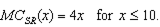 Setting MC equal to p, we can write the firm supply function as x(p)=p/4 -- and adding that over 40 firms, we get the short run market supply function of X(p)=10p. But, with 40 firms and each unable to produce more than 10 units in the short run, this implies the market supply function is
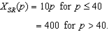
Setting the new demand function equal to this supply function, we get p=35.
In the long run, price has to go back up to 60 (since firm costs have not changed) -- at which price only 100 units are demanded. This implies the number of firms will drop from 40 to 10.
You might also like to view...
The situation in which a firm charges different prices for different blocks of output is referred to as:
A) first-degree price discrimination. B) second-degree price discrimination. C) third-degree price discrimination. D) fourth-degree price discrimination.
We may be tempted to determine the optimal level of advertising expenditures at the point where the last dollar spent on advertising generates an additional dollar of sales revenue (i.e, the marginal revenue of advertising equals one)
In general, this rule will not allow the firm to maximize profits because it ignores the: A) price elasticity of demand. B) marginal cost of additional sales generated by the advertising. C) advertising-to-sales ratio. D) fixed costs of advertising.
If Ellie Mae spends her income on possum and biscuits, and the price of possum is three times the price of biscuits, then when Ellie Mae maximizes total utility, she will buy
a. equal quantities of possum and biscuits b. three times as much possum as biscuits c. three times as many biscuits as portions of possum d. biscuits and possum until the marginal utility of possum is three times the marginal utility of biscuits e. biscuits and possum until the marginal utility of biscuits is three times the marginal utility of possum
Exhibit 2-2 Production possibilities curve In Exhibit 2-2, the opportunity cost of coffee when moving from A to B is:
A. 2 million bushels of corn. B. 6 million bushels of corn. C. 8 million bushels of corn. D. 14 million bushels of corn.