Design a rate feedback controller using root locus techniques for the plant,
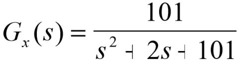
such that the following performance specifications are met:
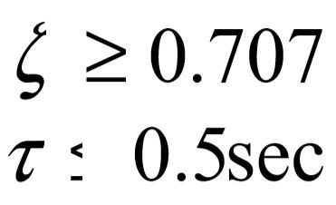
System is stable.
What will be an ideal response?
Given the specifications on the desired closed loop performance in terms of  identify the specification region or point, s*, in the s-plane. The spec region is the cone shown in the following figure.
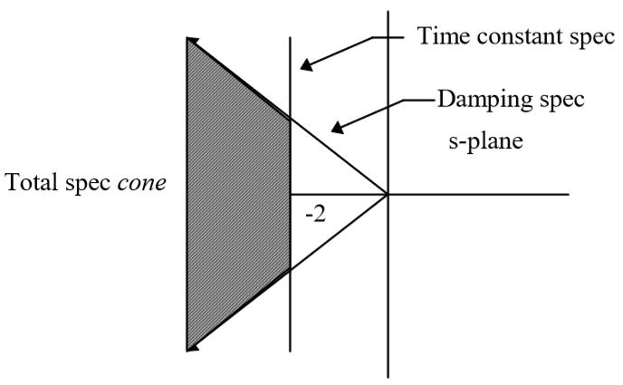
We can design to any point in the total spec cone. For demonstration purposes we will select our design point at the corner of the cone, 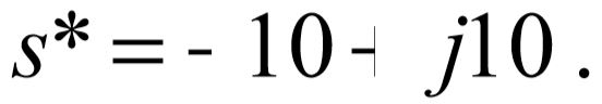
Step 2:
The rate feedback compensator is implemented in the rate feedback configuration shown in the following figure.
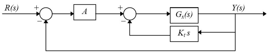
The rate feedback configuration is normally applied to systems which have two outputs, one is the controlled variable and the other is the derivative of the controlled variable. Therefore the inner loop feedback path, Kt s, becomes just Kt , the input is the derivative of the controlled variable.
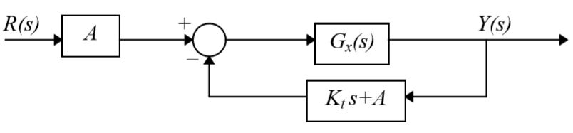
The rate feedback structure can be simplified by moving the A gain leftward through the summing junction and combining the resulting two feedback loops, which are now parallel paths. The simplified diagram is shown below.
The feedback loop transfer function can be factored into monic form to produce,
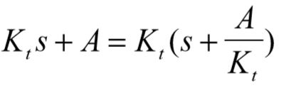
In this form the zero added by the rate feedback configuration can be clearly seen at 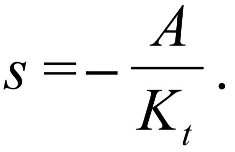
Select the lead zero to move the rightmost pole(s) to s*. The rightmost poles are the dominant poles, that is, they are the poles that govern the fundamental parts of the response. In this example the plant only has two poles located at 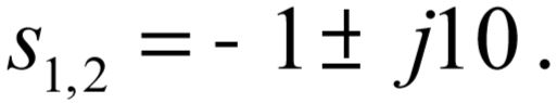 If a zero were placed at about s = –20, the plant poles would tend to travel leftward in a circular path with the center at the zero. Along their trajectory the poles would be dragged through the design point,
 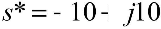 so this zero seems to be satisfactory at this point in the design.
Step 3:
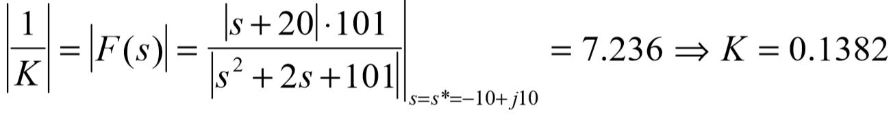
Draw the root locus for 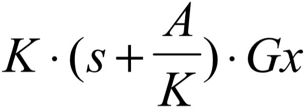 and select K for desired dominant closed loop pole location(s). For brevity we are using K in place of Kt. The gain is calculated below.
Step 4:
Compute A since you know K and (-A/K).
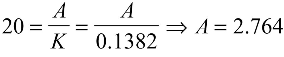
Step 5:
The rate feedback controller is shown in the following figure.
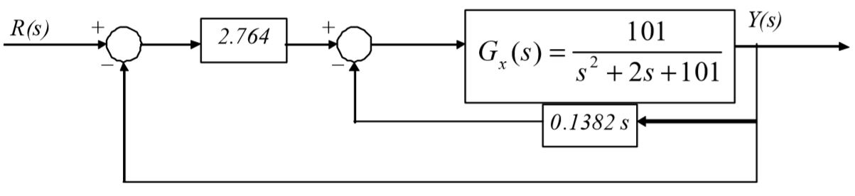
Although the value computed for K is only a starting value, it should be fairly close to the final design value. The design should be simulated to determine whether additional tuning is required.
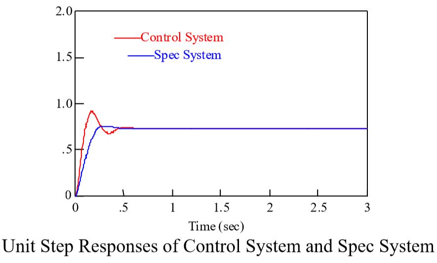
The unit step response of the control system and the spec system, 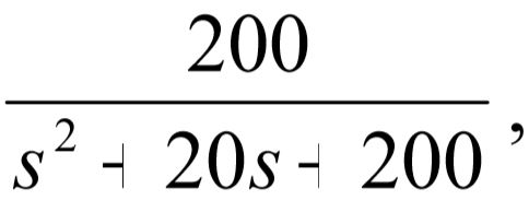 is shown below.
You might also like to view...
The mixture is not stable and forms two liquid phases. One of the phases as a composition of 45% component 1, while other phase has a composition of 15% of component 1.
Consider the figure that provides the molar Gibbs free energy of mixing as a function of composition for a binary mixture.
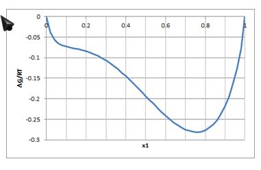
If the overall composition of the mixture is 30% of component 1, is the mixture stable? If not, what are estimates of the compositions of the liquid phases that are in equilibrium?
Which raw materials are used in the manufacturing of Portland cement (PC)?
What will be an ideal response?
NFPA 72® contains requirements for _____.
a. all electrical work performed in a building b. residential and commercial installation of fire alarm systems and equipment c. life safety d. the testing, operation, installation, and periodic preventive maintenance of fire alarm systems
____ reduces the amount of pipe needed to supply fixtures as it saves energy and water by reducing hot water pipe runs.
A. Stacked plumbing B. Layered plumbing C. Double-jointed plumbing D. Pre-plumbing