Compare and contrast the "life cycle" hypothesis and the "permanent income" hypothesis. What are their respective implications for inequality in the income distribution?
Life-cycle variation in income suggests that people's spending patterns vary less over their lifetimes than their income patterns. Young people may borrow so that they can spend more than they earn. An example of this would be a young person borrowing to go to college, buy a car, or buy a house. Annual earnings peak around age 50 . Not surprisingly, many people save more in middle-age than at other times in their life. Their savings allow them to pay off the debts incurred when they were younger and to put away money that they will use to supplement their incomes once they retire.
The permanent income hypothesis tries to account for random and transitory forces that affect income. People may borrow when they experience a temporary reduction in income and may save unexpected increases in income (e.g. a holiday bonus from an employer). The two theories are not mutually exclusive.
Both theories would indicate that standard measures of income distribution overstate inequality in the distribution of well-being.
You might also like to view...
Assuming no change in the effective tax rate on capital, a decrease in the government budget deficit will reduce the current account deficit if and only if the decrease in the budget deficit
A) reduces desired national saving. B) increases desired national saving. C) reduces desired national investment. D) increases desired national investment.
Monetarists assume that suppliers of labor
a. always have perfect information about the real wage. b. base their decisions on the expected real wage. c. may or may not know the real wage. d. could not possibly have perfect information.
The Great Depression:
A. ended a few months after the stock market crash of 1929. B. occurred only in the United States. C. resulted in the development of microeconomics. D. was a period of low production and high unemployment.
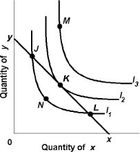 Using the above figure, we can conclude that
A. L is preferred to K. B. the consumer is indifferent between J and M. C. the consumer will purchase goods at combination M. D. K is the optimal combination of goods.