The members of the Greene family refuse to communicate with one another and are constantly bickering. What type of forces is representative of this family?
A. centrifugal
B. central
C. centripetal
D. conforming
a
You might also like to view...
What are some of the concerns of young children?
What will be an ideal response?
Which of the following is an advantage of the mixed method approach to research?
a. The strength of one methodology can potentially overcome a weakness of the other. b. The use of words and narratives can add meaning and insights to numbers generated by the quantitative side. c. The mixed approach is a good way to verify existing theories. d. The mixed approach can provide stronger conclusion and a more complete understanding of a phenomenon through corroboration of findings. e. All of the above.
What research purpose is best suited for quantitative research studies?
a. To understand multiple perspectives and contexts among individuals b. To explore the complexity and meaning of phenomena c. To uncover the unexpected or unique d. To uncover the relationship among specific concepts
How much variance in burnout does the final model explain?
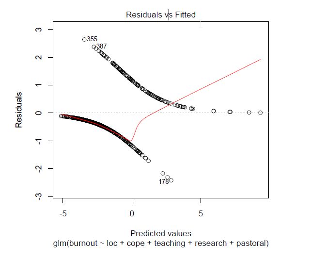
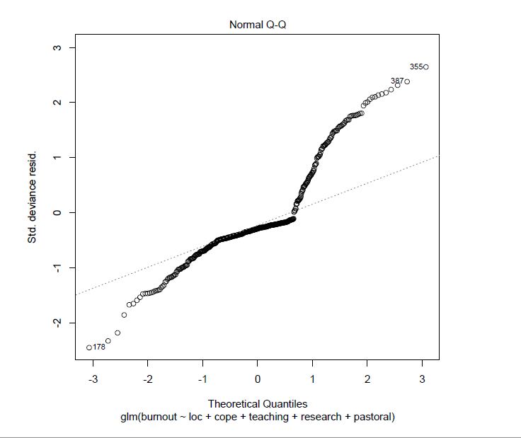
Recent research has shown that lecturers are among the most stressed workers. A researcher wanted to know exactly what it was about being a lecturer that created this stress and subsequent burnout. She recruited 75 lecturers and administered several questionnaires that measured: Burnout (high score = burnt out), Perceived Control (high score = low perceived control), Coping Ability (high score = low ability to cope with stress), Stress from Teaching (high score = teaching creates a lot of stress for the person), Stress from Research (high score = research creates a lot of stress for the person), and Stress from Providing Pastoral Care (high score = providing pastoral care creates a lot of stress for the person). The outcome of interest was burnout, and Cooper’s (1988) model of stress indicates that perceived control and coping style are important predictors of this variable.
The remaining predictors were measured to see the unique contribution of different aspects of a lecturer’s work to their burnout. The R output is below and the remaining questions relate to this output.
summary(burnoutModel.1)
Call:
glm(formula = burnout ~ loc + cope, family = binomial(), data = burnoutData)
Deviance Residuals:
Min 1Q Median 3Q Max
-2.9217 -0.5163 -0.3730 0.1273 2.0848
Coefficients:
Estimate Std. Error z value Pr(>|z|)\
loc 0.061080 0.010915 5.596 2.19e-08 ***
cope 0.082714 0.009369 8.829 < 2e-16 ***
---
Signif. codes: 0 ‘***’ 0.001 ‘**’ 0.01 ‘*’ 0.05 ‘.’ 0.1 ‘ ’ 1
(Dispersion parameter for binomial family taken to be 1)
Null deviance: 530.11 on 466 degrees of freedom
Residual deviance: 364.18 on 464 degrees of freedom
AIC: 370.18
Number of Fisher Scoring iterations: 5
logisticPseudoR2s(burnoutModel.1)
Pseudo R^2 for logistic regression
Hosmer and Lemeshow R^2 0.313
Cox and Snell R^2 0.299
Nagelkerke R^2 0.441
exp(burnoutModel.1$coefficients)
(Intercept) loc cope
0.01128261 1.06298389 1.08623164
exp(confint(burnoutModel.1))
2.5 % 97.5 %
(Intercept) 0.005160721 0.02292526
loc 1.041229885 1.08691181
cope 1.067210914 1.10722003
summary(burnoutModel.2)
Call:
glm(formula = burnout ~ loc + cope + teaching + research + pastoral,
family = binomial(), data = burnoutData)
Deviance Residuals:
Min 1Q Median 3Q Max
-2.41592 -0.48290 -0.28690 0.02966 2.63636
Coefficients:
Estimate Std. Error z value Pr(>|z|)
(Intercept) -4.43993 1.08565 -4.090 4.32e-05 ***
loc 0.11079 0.01494 7.414 1.23e-13 ***
cope 0.14234 0.01639 8.684 < 2e-16 ***
teaching -0.11216 0.01977 -5.673 1.40e-08 ***
research 0.01931 0.01036 1.863 0.062421 .
pastoral 0.04517 0.01310 3.449 0.000563 ***
---
Signif. codes: 0 ‘***’ 0.001 ‘**’ 0.01 ‘*’ 0.05 ‘.’ 0.1 ‘ ’ 1
(Dispersion parameter for binomial family taken to be 1)
Null deviance: 530.11 on 466 degrees of freedom
Residual deviance: 321.20 on 461 degrees of freedom
AIC: 333.2
Number of Fisher Scoring iterations: 6
modelChi; chidf; chisq.prob
[1] 208.9086
[1] 5
[1] 0
logisticPseudoR2s(burnoutModel.2)
Pseudo R^2 for logistic regression
Hosmer and Lemeshow R^2 0.394
Cox and Snell R^2 0.361
Nagelkerke R^2 0.531
exp(burnoutModel.2$coefficients)
(Intercept) loc cope teaching research pastoral
0.01179680 1.11715594 1.15296414 0.89389904 1.01949919 1.04620942
exp(confint(burnoutModel.2))
2.5 % 97.5 %
(Intercept) 0.001317788 0.09419003
loc 1.086274965 1.15212014
cope 1.118430575 1.19286786
teaching 0.858532732 0.92793154
research 0.999115252 1.04068582
pastoral 1.020119629 1.07403586
a. 3.61–5.31%
b. 36.1–53.1%
c. 0.361–0.531%
d. 31.3%